Week Eleven

Week Eleven

Not Shocking People While Generating eNeRgY

Part 1: Strain Gauges:

Problem 1:

Figure 1: Minimum and Maximum Voltages measured (Volts)

Figure 2: Low intensity flipping observation

Figure 3: High Intensity Flipping Observation

Figure 4: Low intensity tapping observation

Figure 5: High Intensity Tapping Observatinon

Problem 2:

Figure 6: Single Sequence tapping output 

Figure 7: Single Sequence Flipping output

Part B:
Problem 1:

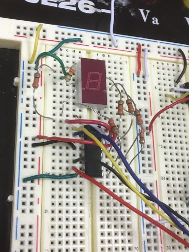
 Figure 8: Rectifier Circuit Setup

Figure 9: Signal Output Snapshot

Problem 2:

Figure 10: Calculated V_rms. Measured values are the same, just not recorded onto table.

Problem 3:

We calculated the RMS values by taking the peak values taken by the oscilloscope and divided the value bu sqrt(2). The measured and calculated values match.

Problem 4:

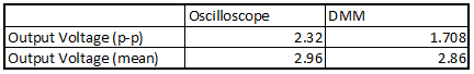
Figure 11: Output Voltages of rectifier in parallel with 1 micro Farad Capacitor

Problem 5: 

Figure 12: Output voltages of rectifier in parallel with 100 micro Farad Capacitor

The peak to peak voltage output is much lower, but the mean output is higher.

Part C: Energy Harvesters

Problem 1:

Figure 13: Final output voltage at duration end using the tapping energy harvester.

Figure 14: Final output voltage at duration end using the flipping strain gauge energy harvester.

Problem 2: With the tapping energy harvester, it seemed that with the initial tap, there was the highest amount of energy. At the start of every test, the energy read about or above 200 mV, however, as time went on and the test continued, the output went down. This is because the more we tapped out harvester, the faster the capacitor was filled which was decreasing the flow change in voltage through the capacitor. 

With the flipping energy harvester was used, the more and longer we flipped the harvester over time the greater the amount of voltage that dropped through the capacitor.

Problem 3: There would be a back-flow of energy due to there not being a diode, which would make the output have negative troughs as well as positive peaks.

Problem 4: 

close all;

clear all;

t = [125 80 0]; %1 Tap/sec

y = [71 91 0]; %4 tap/sec

f = [17 19 71]; %1 flip/sec

g = [105 205 220]; %4 flip/sec

d = [10 20 30];

plot(d,t,'r')

hold on

plot(d,y,':r')

hold on

plot(d,f,'b')

hold on

plot(d,g,':b')

xlabel('Seconds(s)')

ylabel('Output Voltage(mV)')

legend('1 Tap/Second','4 Tap/Second','1 Flip/Second','4 Flip/Second')

Figure 15: Plotted information from Figures 13 and 14.

Week Ten

Not Shocking People Whilst Using MATLAB

Week Ten

%1 

clear all;
close all;
x = [1 2 3 4 5];
y = 2.^x;
plot(x, y, 'LineWidth', 6)
xlabel('Numbers', 'FontSize', 12)
ylabel('Results', 'FontSize', 12)

clear all; %2 clear all removes prior variable and function definitions

close all; %3 closes any prior command based windows (i.e. plot, ext.)

x = [1 2 3 4 5]; 

y = 2.^x;

plot(x, y, 'LineWidth', 6)

xlabel('Numbers', 'FontSize', 12)

ylabel('Results', 'FontSize', 12)

%4 when typing x and pressing enter, the prior logged values for x appear

%the matrix has one row and five colomns.

%5 the semicolon is used when defining the function, which without it, would

%the values would not be stored and the plot function nor defined

%6 If a . is not used before the power, the x values will be read as a whole

%matrix instead of being recognized individually.

%7 It affects the thickness of the line that is plotted

%8

clear all; 

close all; 

x = [1 2 3 4 5];

y = 2.^x;

plot(x, y, '-rO','LineWidth', 5,'markersize',18)

xlabel('Numbers', 'FontSize', 12)

ylabel('Results', 'FontSize', 12)

%9

clear all; 

close all; 

x = [1; 2; 3; 4; 5;];

y = 2.^x;

plot(x, y, '-rO','LineWidth', 5, 'markersize',18)

xlabel('Numbers', 'FontSize', 12)

ylabel('Results', 'FontSize', 12)

%The plot stays the same, as these colons are already expressed when the .

%is placed before the ^

%10

clear all; 

close all; 

x = [1 2 3 4 5];

y = 2.^x;

plot(x, y, ':ks','LineWidth', 6, 'markersize',14)

grid on

xlabel('Numbers', 'FontSize', 12)

ylabel('Results', 'FontSize', 12)

%11

%a : on google calculator

%sin(30)=0.5

%b

%sin(30) = -0.9880

%They are differenct because google automatically calculates sin using

%degree values inside the parenthesis, whereas when in MATLAB, sin(x) is a

%radian command, while sind(x) is using degrees

%c

%sind(30) = 0.5000

%12

clear all;

close all;

t = linspace(0,0.12,10);

y = 10*sin(100*t);

u = linspace(0,0.12,1000);

z = 10*sin(100*u);

plot(t,y,'-ro')

hold on

plot(u,z,'-k')

xlabel('Time(s)')

ylabel('y function')

legend('Course','Fine')

%13 

%Differences: Two plots were formatted atop one another using the hold on

%command, the variables were defined using intervals of range of values,

%there was a legend added.

%14
clear all;
close all;
t = linspace(0,0.12,10);
y = 10*sin(100*t);
u = linspace(0,0.12,1000);
z = 10*sin(100*u);
f=find(z>5)
z(f)=5
plot(t,y,'-ro')
hold on
plot(u,z,'-k')

xlabel('Time(s)')
ylabel('y function')
legend('Course','Fine')

PART B

1.

2.

%PART B

%2

clear all;

close all;

f=[.1 .2 .3 .4 .5 .6 .7 .8 .9 1 1.1 1.2 1.3 1.4 1.5 1.6 1.7 1.8 1.9 2]

v=[3.25 3.82 3.66 3.58 3.5 3.4 3.3 3.2 3.07 2.96 2.85 2.75 2.63 2.53 2.45 2.35 2.28 2.2 2.12 2.05]

plot(f,v,'-ro')

xlabel('frequency(KHz)')

ylabel('V out(V)')

grid on

3.

fc= 1/(2*3.141593*7500*0.000000022)

fc =

  964.5753

%The voltage at 965 is 3

clear all;

close all;

f=[.1 .2 .3 .4 .5 .6 .7 .8 .9 1 1.1 1.2 1.3 1.4 1.5 1.6 1.7 1.8 1.9 2];

v=[3.25 3.82 3.66 3.58 3.5 3.4 3.3 3.2 3.07 2.96 2.85 2.75 2.63 2.53 2.45 2.35 2.28 2.2 2.12 2.05];

c=find(v>3)

v(c)=3

plot(f,v,'-ro')

xlabel('frequency(KHz)')

ylabel('V out(V)')

grid on

%4

clear all;

close all;

f=[.1 .2 .3 .4 .5 .6 .7 .8 .9 1 1.1 1.2 1.3 1.4 1.5 1.6 1.7 1.8 1.9 2];

v=[3.25 3.82 3.66 3.58 3.5 3.4 3.3 3.2 3.07 2.96 2.85 2.75 2.63 2.53 2.45 2.35 2.28 2.2 2.12 2.05];

c=find(v>3)

v(c)=3

plot(f,v,'-ro')

hold on

y=[.1 .2 .3 .4 .5 .6 .7 .8 .9 1 1.1 1.2 1.3 1.4 1.5 1.6 1.7 1.8 1.9 2];

u=[3.25 3.82 3.66 3.58 3.5 3.4 3.3 3.2 3.07 2.96 2.85 2.75 2.63 2.53 2.45 2.35 2.28 2.2 2.12 2.05];

plot(y,u,'--k')

legend('output with cutoff','output')

xlabel('frequency(KHz)')

ylabel('V out(V)')

grid on

%5

%1 & 3

%2

clc;

clear all;

close all;

f=[.1 .2 .3 .4 .5 .6 .7 .8 .9 1 1.1 1.2 1.3 1.4 1.5 1.6 1.7 1.8 1.9 2]

v=[3.25 3.82 3.66 3.58 3.5 3.4 3.3 3.2 3.07 2.96 2.85 2.75 2.63 2.53 2.45 2.35 2.28 2.2 2.12 2.05]

plot(f,v,'-ro')

xlabel('frequency(KHz)')

ylabel('V out(V)')

Week Nine

Not Shocking People After Spring Break

Week Nine

1. Measure the resistance of the speaker.

We measured 8.6 Ohms, while online is says this model of speaker offers 32 Ohms.

2. Build the following circuit using a function generator setting the amplitude to 5V (0V offset). What happens when you change the frequency? (video)

Figure 1: Frequency of AC Voltage applied to a speaker.

Figure 2: Circuit Layout

Figure 3: Frequencies compared speaker output.

3. Add one resistor to the circuit in series with the speaker (first 47 Ω, then 820 Ω). Measure the voltage across the speaker. Briefly explain your observations.

Figure 4: Observations while placing resistors in parallel with speaker. The higher the resistor, the lower the amplitude. Therefore, the lower the volume.

4. Build the following circuit. Add a resistor in series to the speaker to have an equivalent resistance of 100 Ω. Note that this circuit is a high pass filter. Set the amplitude of the input signal to 8 V. Change the frequency from low to high to observe the speaker sound. You shouldnot hear anything at the beginning and start hearing the sound after a certain frequency. Use 22 nF for the capacitor.

a.

Figure 5: Video explaining the operation of the high pass  filter connected to the speaker.

b. & c.

Figure 6: V_out measured and V_out/V_in Calculated with respect to frequency increasing.

d. It looks like the cutoff frequency is 5000 with the voltage V_out capping off at 0.014V.
e. 

Figure 7: Plot of Frequency v. Output. The climax of the curve shows the critical frequency of the circuit.

f. The Cutoff Frequency according to our plot and theoretical calculations is 5000 Hz.

g. As the frequency increases, to a high 2000 Hz, the voltage amplitude takes on a significant enough value to be audible to human ears. However, when the frequency reaches 5000 Hz, the voltage reaches its cutoff point and begins to decrease. 

5. Design the circuit in 4 to act as a low pass filter and show its operation. Where would you put the speaker? Repeat 4a-g using the new designed circuit.

We would place the speaker in parallel with a capacitor, the pair of which would be in series with a resistor. 

a.

Figure 8: Video explaining the operation of the low pass filter.

b. & c.

Figure 9:V_out measured and V_out/V_in Calculated with respect to frequency increasing in a low pass circuit.

d. The cutoff frequency is at 1000, capping off at .596 V.

e.

Figure 10: Plot of Frequency v. Output of a low pass circuit. The climax of the curve shows the critical frequency of the circuit.

f. According to the plot, our cutoff frequency is at 1000.

g. The low pass filter works in a way where the capacitor works as an extremely high resistance to low frequency signals, making them pass to the speaker, whereas high frequency will pass through the capacitor, and not to the speaker, as can be seen above. 

6. Construct the following circuit and test the speaker with headsets. Connect the amplifier output directly to the headphone jack (without the potentiometer). Load is the headphone jack in the schematic. “Speculate” the operation of the circuit with a video.

Figure 11: Video with speculation of the operation of the circuit.

Week Eight

Week Eight

NOT SHOCKING PEOPLE

Steps of Rube Goldberg Circuit

Figure 1: Video of Rube Goldberg Function

Circuit Explanation

Figure 2: Step 1: The Pressure sensor is pressed by a weighted object.

Figure 3: Step 2: The light of the LED connected to the OR gate turns on, informing the user that we must begin applying heat to the temperature sensor. 

Figure 4: The gate mentioned in step 2

Figure 5: Image of AND gate on bottom and driver on top. The and gate inputs are connected to the relay input is parallel and the pressure sensor. When both of these are active the counter will begin to function.

Figure 6: Step 3: The heat provided to the temperature sensor allows for a voltage and  current to flow into the ompamp, amplifying the current, allowing the relay to switch on. 

Figure 7: Step 4: Once the and gate is satisfied with two active inputs, then the driver begins to send signals to the counter, which then sends signal to the digital display, starting the count up from 0 to 9 and then repeating.

Figure 8: Step 5: Once the relay is active, current is applied to a motor which spins this mechanical apparatus, knocking over something important and making something happen for somebody else.

Struggles

One struggle we faced was getting the relay to switch while connected to the temperature sensor. We noticed that there was not enough voltage going between the temperature sensor output to the relay (only 1V). We first tried to fix this with a 741 amplifier being placed between the two, but that did not amplify the current enough to switch on the relay. Instead, we used an opamp to amplify, which introduced our next problem.

Another struggle we faced was applying the proper gain to the opamp to switch the relay on, even though we knew it could work, we were concerned why it wasn't. What we had found was that we were applying too small of a voltage to the voltage input to power the opamp. After increasing the opamp voltage to 20 V, the amplified voltage and current was able to reach the appropriate amplitude to switch the relay on.